출처
코드로 방정식 표현하기
- 기존의 파이썬 코드로 수식을 표편하는 것은 너무 느림
- 그래서 Numpy를 씀
Numpy
- Numerical Python
- 파이썬의 고성능 과학 계산용 패키지
- Matrix와 Vector와 같은 Array 연산의 사실상 표준
- 일반 List에 비해 빠르고 메모리 효율적
- 반복문 없이 데이터 배열에 대한 처리를 지원함
- 선형대수와 관련된 다양한 기능을 제공함
- C, C++, 포트란 등의 언어와 통합 가능
Numpy Install
ndarray
import
- numpy의 호출 방법
- 일반적으로 numpy는 np라는 alias(별칭) 이용해서 호출
Array creation
import numpy as np
test_array = np.array([1,4,5,8],float)
print(test_array)
type(test_array[3])
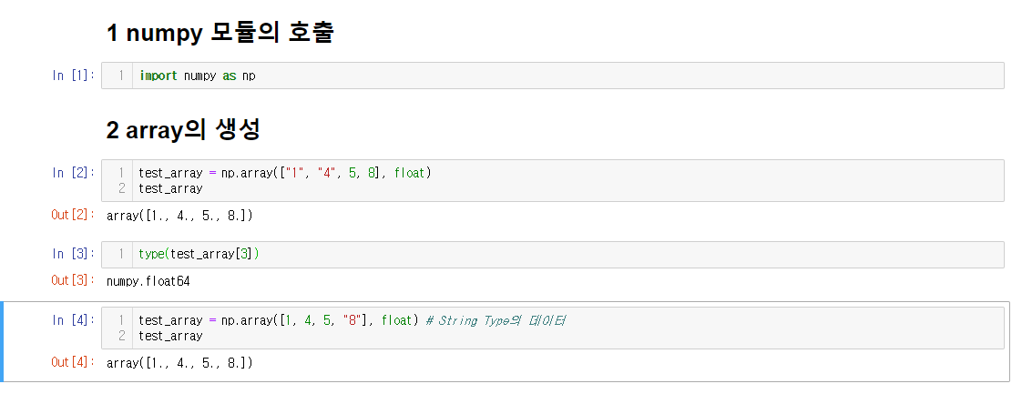
- numpy는 np.array 함수를 활용하여 배열을 생성함 –> ndarray
- numpy는 하나의 데이터 type만 배열에 넣을 수 있음
- List와 가장 큰 차이점, Dynamic typing not supported
- C의 Array를 사용하여 배열을 생성함
- float64는 64비트라는 뜻
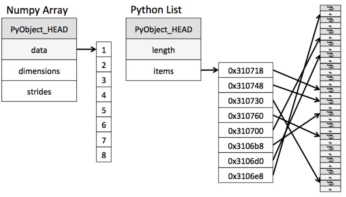
Numpy와 Python List의 배열 저장방식 차이
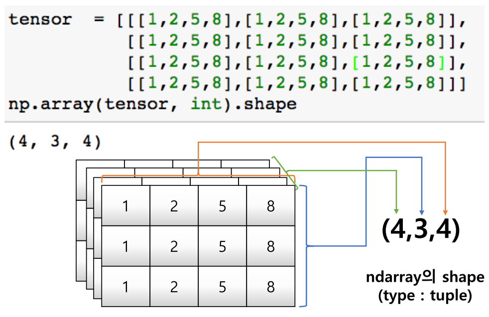
shape
- numpy array의 object의 dimension을 반환함
test_array1 = np.array([1, 4, 5, "8"], float)
test_array2 = np.array([[1, 4, 5, 8], [2, 4, 6, 8]], float)
test_array1.shape
test_array2.shape
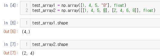
- shape 결과로 나온 값은 dimension이 추가될 수록 하나씩 밀림
- (4, ) –> (3, 4) –> (4, 3, 4)…
ndim(number of dimension) 와 size
- data type은 float32나 float64를 씀
shape handling
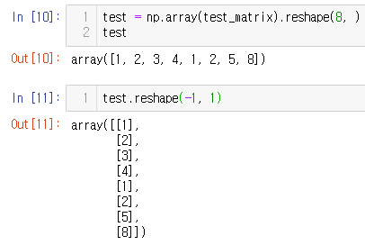
reshape
- Array의 shape의 크기를 변경함 (element의 개수는 동일)
test_matrix = [[1, 2, 3, 4], [1, 2, 5, 8]]
np.array(test_matrix).shape
np.array(test_matrix).reshape(2,2,2)
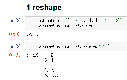
- reshape 인자에 -1을 넣으면 row나 column의 개수를 기반으로 자동으로 개수 설정
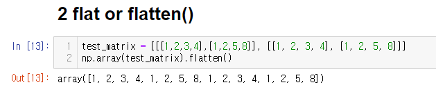
flatten
test_matrix = [[[1,2,3,4],[1,2,5,8]], [[1, 2, 3, 4], [1, 2, 5, 8]]]
np.array(test_matrix).flatten()
Indexing and Slicing
Indexing
a = np.array([[1, 2, 3], [4.5, 5, 6]], int)
print(a)
print(a[0,0]) # Two dimensional array representation #1
print(a[0][0]) # Two dimensional array representation #2

a[0,0] = 12 # Matrix 0,0에 12 할당
print(a)
a[0][0] =5 # Matrix 0,0에 5 할당
print(a)
- List와 달리 이차원 배열에서 [0, 0]과 같은 표기법을 제공함
- Matrix일 경우 앞은 row 뒤는 column을 의미함
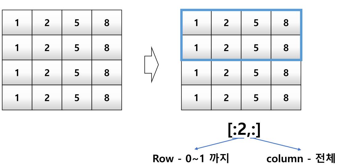
slicing
a = np.array([[1, 2, 3, 4, 5], [6, 7, 8, 9, 10]], int)
a[:,2:] # 전체 Row의 2열 이상
a[1, 1:3] # 1 Row의 1열 ~ 2열
a[1:3] # 1 Row ~ 2 Row의 전체
- List와 달리 행과 열 부분을 나눠서 slicing이 가능함
- Matrix의 부분 집합을 추출할 때 유용함
create function
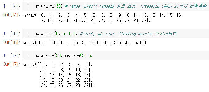
arange
np.arange(30) # range: List의 range와 같은 효과, integer로 0부터 29까지 배열추출
np.arange(0, 5, 0.5) # 시작, 끝, step, floating point도 표시가능함
np.arange(30).reshape(5, 6)
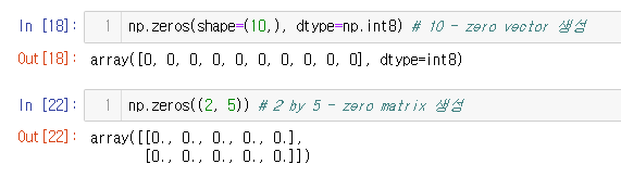
zeros
np.zeros(shape=(10,), dtype=np.int8) # 10 - zero vector 생성
np.zero((2.5)) # 2 by 5 - zero matrix 생성
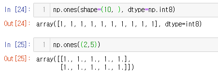
ones
np.ones(shape=(10, ), dtype=np.int8)
np.ones((2, 5))
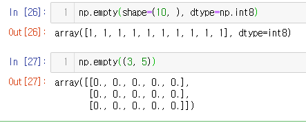
empty
- shape만 주어지고 비어있는 ndarray 생성인데 memory initialization이 되지 않음
np.empty(shape=(10, ), dtype=np.int8)
np.empty((3, 5))
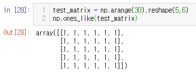
something_like
- 기존 ndarray의 shape 크기 만큼 1, 0 또는 empty array를 반환
test_matrix = np.arange(30).reshape(5,6)
np.ones_like(test_matrix) # 1로 채워라
- 딥러닝에서 은근 쓰임
- 딥러닝은 numpy에서 미분 가능하게 한 것
- numpy의 기본적인 옵션이 그래서 tensorflow에 다 있음
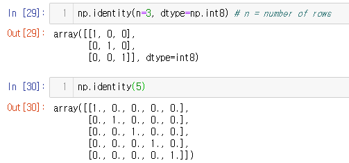
identity
np.identity(n=3, dtype=np.int8) # n = number of rows
np.identity(5)
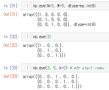
eye
- 대각선이 1인 행렬, k값의 시작 index의 변경이 가능
np.eye(N=3, M=5, dtype=np.int8)
np.eye(3)
np.eye(3, 5, k=2) # k는 start index
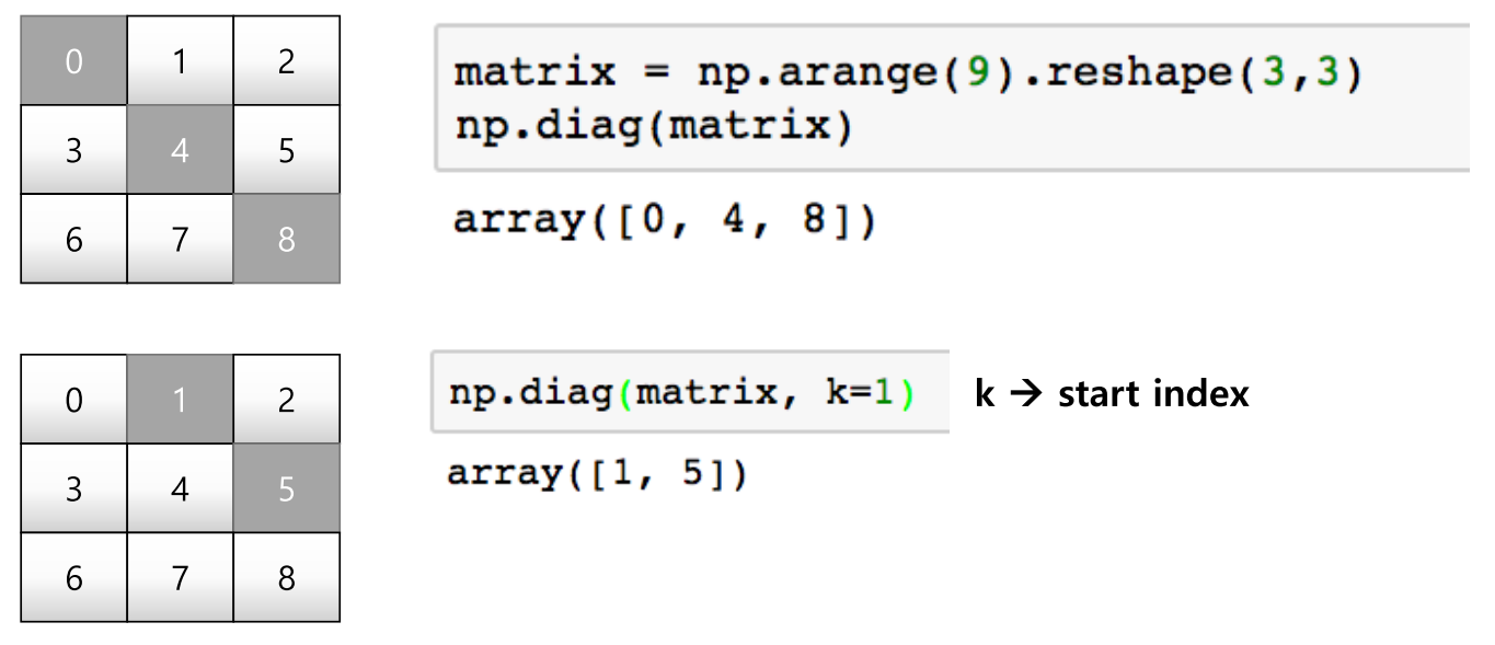
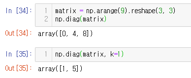
diag
matrix = np.arange(9).reshape(3, 3)
np.diag(matrix)
np.diag(matrix, k=1)
random sampling
- 데이터 분포에 따른 sampling으로 array를 생성
np.random.uniform(0, 1, 10).reshape(2, 5) # 균등분포
np.random.normal(0, 1, 10).reshape(2, 5) # 정규분포
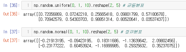
- 분포에 따른 값을 array로 만들 수 있다정도로 기억
operation functions
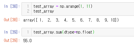
sum
- ndarray의 element들 간의 합을 구함, list의 sum 기능과 동일
test_array = np.arange(1, 11)
test_array
test_array.sum(dtype=np.float)
axis
- 모든 operation function을 실행할 때 기준이 되는 dimension 축
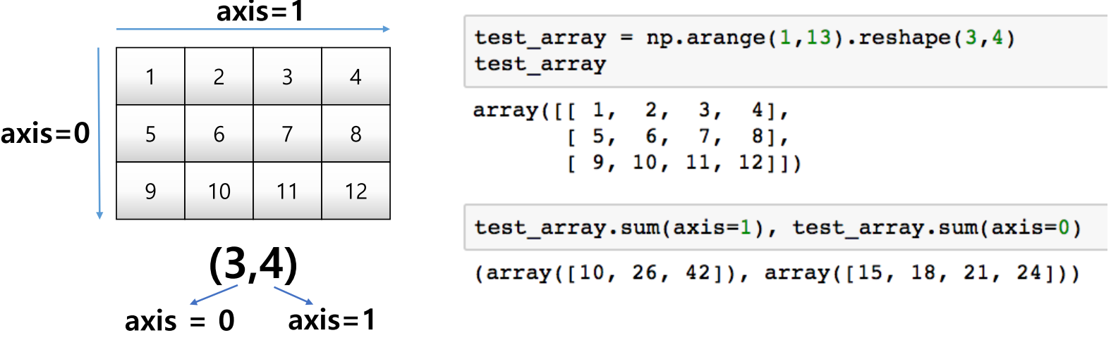
test_array = np.arange(1, 13).reshape(3, 4)
test_array
test_array.sum(axis=1), test_array.sum(axis=0)
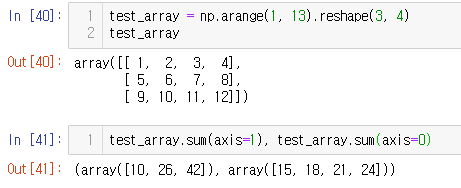
- 새로 생기는 부분이 axis 0이 되는 것을 기억하면 됨
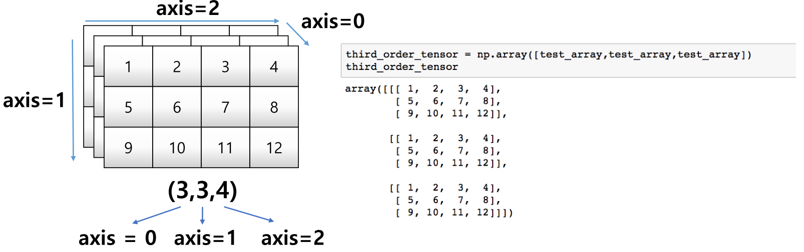
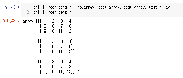
third_order_tensor = np.array([test_array, test_array, test_array])
third_order_tensor
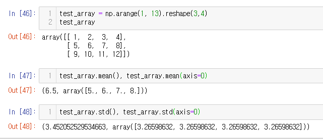
mean & std
- ndarray의 element들 간의 평균 또는 표준편차를 반환
test_array = np.arange(1, 13).reshape(3,4)
test_array
test_array.mean(), test_array.mean(axis=0)
test_array.std(), test_array.std(axis=0)
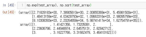
Mathematical functions
exponential
- exp, expm1, exp2, log, log10, log1p, log2, power. sqrt
trigonometric
- sin, cos, tan, acsin, arccos, atctan
hyperbolic
- sinh, cosh, tanh, acsinh, arccosh, atctanh
np.exp(test_array), np.sqrt(test_array)
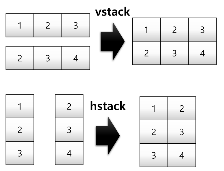
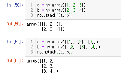
concatenate
a = np.array([1, 2, 3])
b = np.array([2, 3, 4])
np.vstack((a, b))
a = np.array([[1], [2], [3]])
b = np.array([ [2], [3], [4]])
np.hstack((a, b))
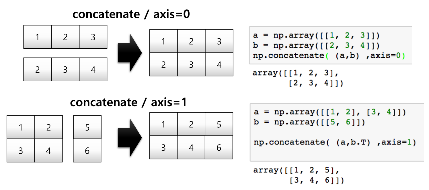
a = np.array([[1, 2, 3]])
b = np.array([[2, 3, 4]])
np.concatenate((a, b), axis = 0)
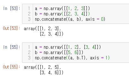
a = np.array([[1, 2], [3, 4]])
b = np.array([[5, 6]])
np.concatenate((a, b.T), axis = 1)
array operation
Operations b/t arrays
- Numpy는 array간의 기본적인 사칙연산을 지원함
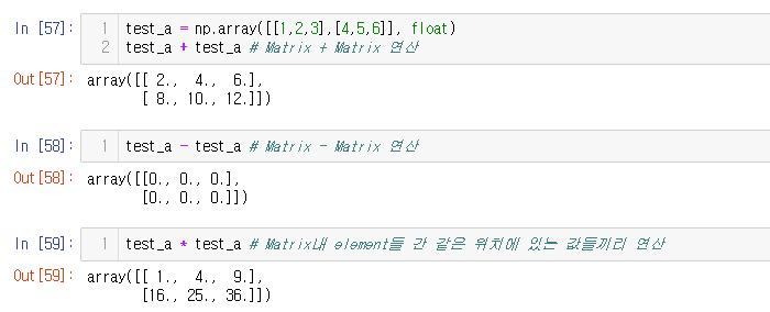
test_a = np.array([[1,2,3],[4,5,6]], float)
test_a + test_a # Matrix + Matrix 연산
test_a - test_a # Matrix - Matrix 연산
test_a * test_a # Matrix내 element들 간 같은 위치에 있는 값들끼리 연산
Element-wise operations
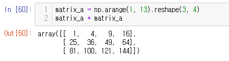
- Array간 shape이 같을 때 일어나는 연산
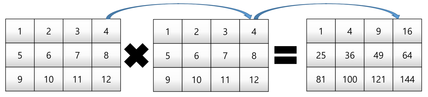
matrix_a = np.arange(1, 13).reshape(3, 4)
matrix_a * matrix_a
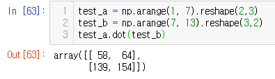
Dot product
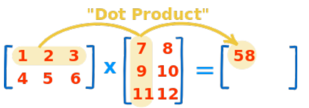
test_a = np.arange(1, 7).reshape(2,3)
test_b = np.arange(7, 13).reshape(3,2)
test_a.dot(test_b)
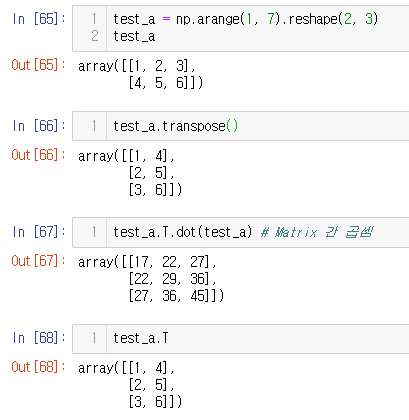
Transpose
- transpose 또는 T attribute 사용
test_a = np.arange(1, 7).reshape(2, 3)
test_a
test_a.transpose()
test_a.T.dot(test_a) # Matrix 간 곱셈
test_a.T
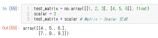
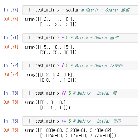
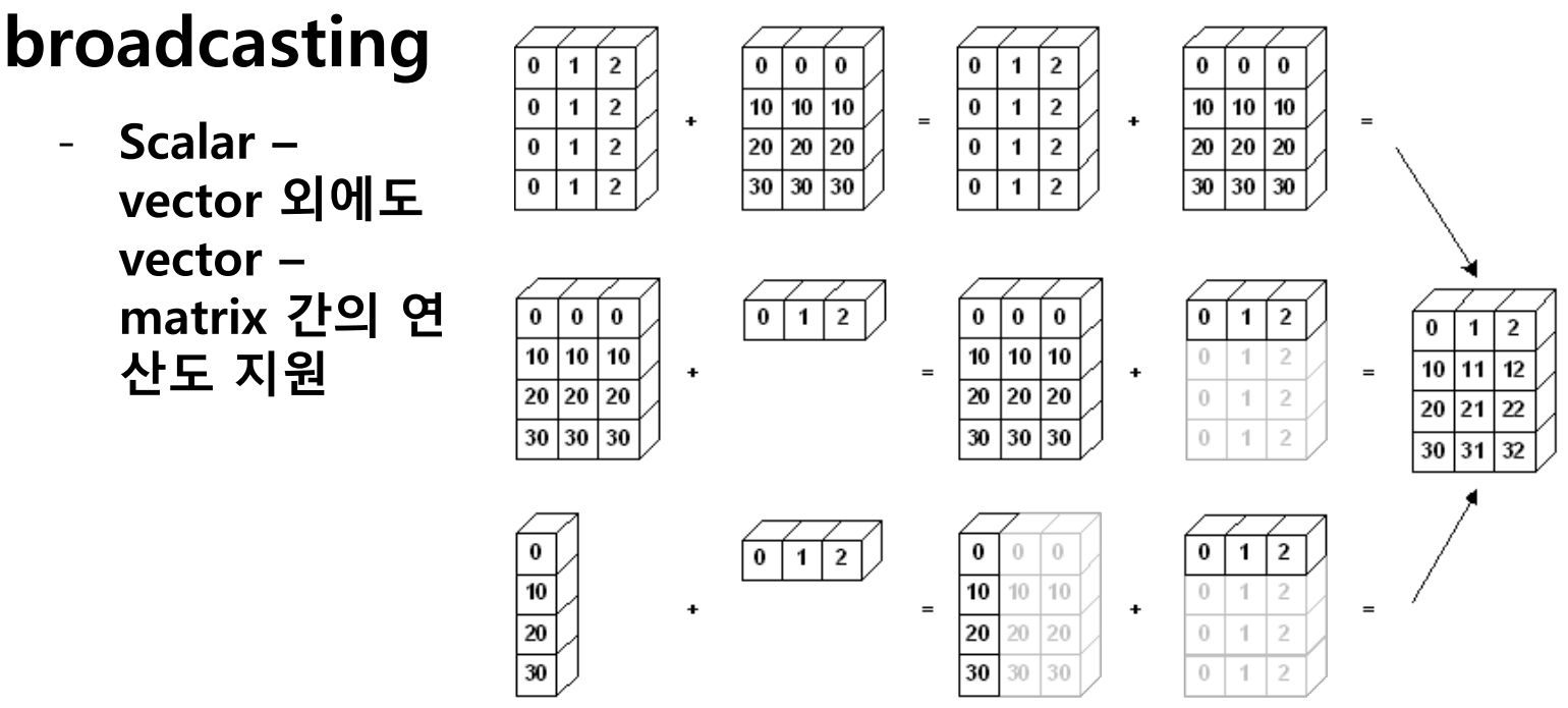
broadcasting
- Shape이 다른 배열 간 연산을 지원하는 기능

test_matrix = np.array([[1, 2, 3], [4, 5, 6]], float)
scalar = 3
test_matrix + scalar # Matrix - Scalar 덧셈
test_matrix - scalar # Matrix - Scalar 뺄셈
test_matrix * 5 # Matrix - Scalar 곱셈
test_matrix / 5 # Matrix - Scalar 나눗셈
test_matrix // 5 # Matrix - Scalar 몫
test_matrix ** 5 # Matrix - Scalar 제곱
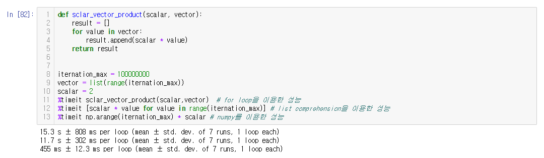
def sclar_vector_product(scalar, vector):
    result = []
    for value in vector:
        result.append(scalar * value)
    return result


iternation_max = 100000000
vector = list(range(iternation_max))
scalar = 2
%timeit sclar_vector_product(scalar,vector)  # for loop을 이용한 성능
%timeit [scalar * value for value in range(iternation_max)] # list comprehension을 이용한 성능
%timeit np.arange(iternation_max) * scalar # numpy를 이용한 성능
- timeeit: jupyter 환경에서 코드의 퍼포먼스를 체크하는 함수
- numpy > list comprehension > for loop 순으로 빠름
- concat 시 numpy는 느림
comparisons
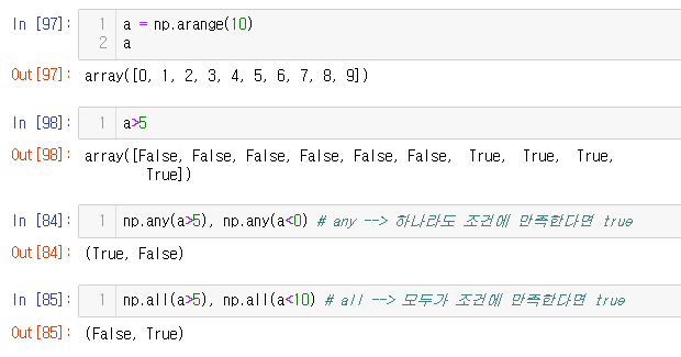
All & Any
- Array의 데이터 전부(and) 또는 일부(or)가 조건에 만족 여부 반환
a = np.arange(10)
a
a>5
np.any(a>5), np.any(a<0) # any --> 하나라도 조건에 만족한다면 true
np.all(a>5), np.all(a<10) # all --> 모두가 조건에 만족한다면 true
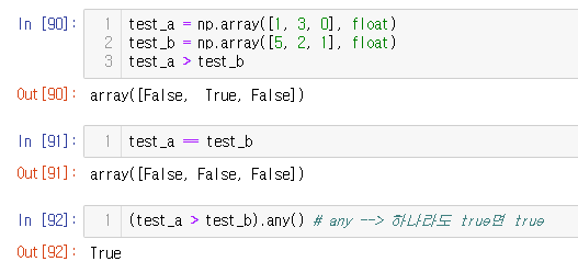
Comparison operation #1
- Numpy는 배열의 크기가 동일할 때 element간 비교의 결과를 Boolean type으로 반환하여 돌려줌
test_a = np.array([1, 3, 0], float)
test_b = np.array([5, 2, 1], float)
test_a > test_b
test_a == test_b
(test_a > test_b).any() # any --> 하나라도 true면 true
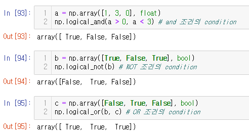
Comparison operation #2
a = np.array([1, 3, 0], float)
np.logical_and(a > 0, a < 3) # and 조건의 condition
b = np.array([True, False, True], bool)
np.logical_not(b) # NOT 조건의 condition
c = np.array([False, True, False], bool)
np.logical_or(b, c) # OR 조건의 condition
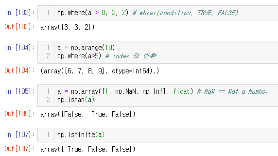
np.where
np.where(a > 0, 3, 2) # whrer(condition, TRUE, FALSE)
a = np.arange(10)
np.where(a>5) # Index 값 반환
a = np.array([1, np.NaN, np.Inf], float) # NaN == Not a Number
np.isnan(a)
np.isfinite(a)
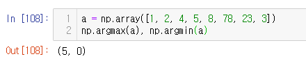
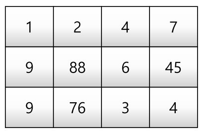
argmax & argmin
- array내 최댓값 또는 최솟값의 index를 반환함
a = np.array([1, 2, 4, 5, 8, 78, 23, 3])
np.argmax(a), np.argmin(a)
a = np.array([[1, 2, 4, 7], [9, 88, 6, 45], [9, 76, 3, 4]])
np.argmax(a, axis=1), np.argmin(a, axis=0)
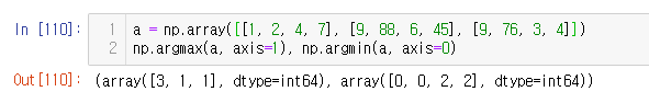
boolean index
- numpy의 배열은 특정 조건에 따른 값을 배열 형태로 추출할 수 있음
- Comparison operation 함수들도 모두 사용 가능
test_array = np.array([1, 4, 0, 2, 3, 8, 9, 7], float)
test_array > 3
test_array[test_array > 3] # 조건이 True인 index의 element만 추출
condition = test_array < 3
test_array[condition]
- index가 아니라 값을 뽑아오는 것을 잊지 마십쇼
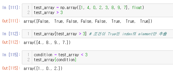
fancy index
- numpy에서 array를 index value로 사용해서 값을 추출하는 방법
a = np.array([2, 4, 6, 8], float)
b = np.array([0, 0, 1, 3, 2, 1], int) # 반드시 integer로 선언
a[b] # bracket index, b 배열의 값을 index로 하여 a의 값들을 추출함
a.take(b) # take 함수: bracket index와 같은 효과
- 추천 관련 공부를 할 때 자주 사용하는 기법
- take 함수 쓰는 것을 권장
numpy data i/o
loadtxt & savetxt
- Text type의 데이터를 읽고 저장하는 기능
# year	hare	lynx	carrot
1900	30e3	4e3	48300
1901	47.2e3	6.1e3	48200
1902	70.2e3	9.8e3	41500
1903	77.4e3	35.2e3	38200
1904	36.3e3	59.4e3	40600
1905	20.6e3	41.7e3	39800
1906	18.1e3	19e3	38600
1907	21.4e3	13e3	42300
1908	22e3	8.3e3	44500
1909	25.4e3	9.1e3	42100
1910	27.1e3	7.4e3	46000
1911	40.3e3	8e3	46800
1912	57e3	12.3e3	43800
1913	76.6e3	19.5e3	40900
1914	52.3e3	45.7e3	39400
1915	19.5e3	51.1e3	39000
1916	11.2e3	29.7e3	36700
1917	7.6e3	15.8e3	41800
1918	14.6e3	9.7e3	43300
1919	16.2e3	10.1e3	41300
1920	24.7e3	8.6e3	47300
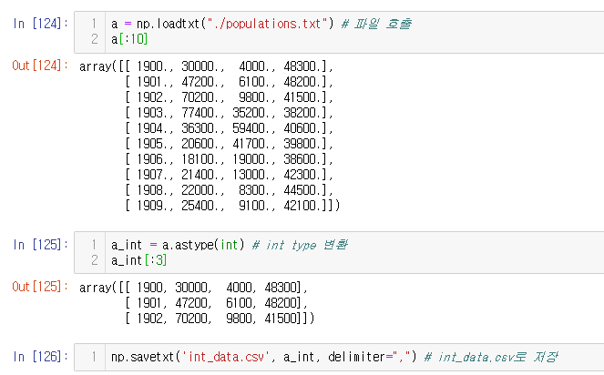
a = np.loadtxt("./populations.txt") # 파일 호출
a[:10]
a_int = a.astype(int) # int type 변환
a_int[:3]
np.savetxt('int_data.csv', a_int, delimiter=",") # int_data.csv로 저장
1.90E+03	3.00E+04	4.00E+03	4.83E+04
1.90E+03	4.72E+04	6.10E+03	4.82E+04
1.90E+03	7.02E+04	9.80E+03	4.15E+04
1.90E+03	7.74E+04	3.52E+04	3.82E+04
1.90E+03	3.63E+04	5.94E+04	4.06E+04
1.91E+03	2.06E+04	4.17E+04	3.98E+04
1.91E+03	1.81E+04	1.90E+04	3.86E+04
1.91E+03	2.14E+04	1.30E+04	4.23E+04
1.91E+03	2.20E+04	8.30E+03	4.45E+04
1.91E+03	2.54E+04	9.10E+03	4.21E+04
1.91E+03	2.71E+04	7.40E+03	4.60E+04
1.91E+03	4.03E+04	8.00E+03	4.68E+04
1.91E+03	5.70E+04	1.23E+04	4.38E+04
1.91E+03	7.66E+04	1.95E+04	4.09E+04
1.91E+03	5.23E+04	4.57E+04	3.94E+04
1.92E+03	1.95E+04	5.11E+04	3.90E+04
1.92E+03	1.12E+04	2.97E+04	3.67E+04
1.92E+03	7.60E+03	1.58E+04	4.18E+04
1.92E+03	1.46E+04	9.70E+03	4.33E+04
1.92E+03	1.62E+04	1.01E+04	4.13E+04
1.92E+03	2.47E+04	8.60E+03	4.73E+04
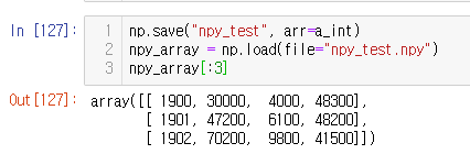
numpy object - npy
- Numpy object (pickle) 형태로 데이터를 저장하고 불러옴
- Binary 파일 형태로 저장함
np.save("npy_test", arr=a_int)
npy_array = np.load(file="npy_test.npy")
npy_array[:3]
Comments